How the competitive exclusion principle can be validated using optical density measurements collected on artificially reconstituted soil ecosystems

Miled EL Hajji; Miled EL Hajji

ISSN: 2690-0777

Open Journal of Environmental Biology

Research Article Open Access Peer-Reviewed

How the competitive exclusion principle can be validated using optical density measurements collected on artificially reconstituted soil ecosystems

Miled EL Hajji*

Author and article information

ENIT-LAMSIN, BP. 37, 1002 Tunis-Belvédère, Tunis El Manar University, Tunis, Tunisia

*Corresponding author: Miled El Hajji, ENIT-LAMSIN, BP. 37, 1002 Tunis-Belvédère, Tunis El Manar University, Tunis, Tunisia, E-mail: miled.elhajji@enit.rnu.tn

DOI: 10.17352/ojeb.000009

Received:05 January, 2019 | Accepted: 18 February, 2019 | Published: 19 February, 2019

Keywords: Modelling; Soil strains; Batch culture; Optical density; Cell recycling; Competition; Least squares method

Cite this as

Hajji ME (2019) How the competitive exclusion principle can be validated using optical density measurements collected on artificially reconstituted soil ecosystems. Open J Environ Biol 4(1): 001-006. DOI: 10.17352/ojeb.000009

Abstract

A mathematical model, validated on experimental data aiming at describing and predicting soil bacteria growth on an essential limited substrate in batch pure cultures is proposed as an extension of the Monod’s one in revisiting the way where the optical density is modelled. This model takes into account viable cell growth, substrate consumption, cell mortality, non-viable cell accumulation in the culture medium and partial dead cell recycling into substrate. The least squares method is used to identify model parameters. The model is extended and validated for mixed cultures proving, for artificially reconstituted soil ecosystems, that there is only competition for the substrate.

Mathematics Subject Classification: 34D23, 35N25, 37B25, 49K40, 00A71.

Main article text

Introduction

Microbial world is very complex by its taxonomic and functional diversity and by the ubiquity of the microorganisms spread in the different ecosystems at the surface of the earth. Such ubiquity resulted from the various colonisation strategies of microbes based on their high ability to use a wide range of substrate in different physico-chemical niches. In environmental matrices, microbial communities are considered as a complex assemblage of a huge taxonomic and functional diversity of populations and several studies describe population dynamics as well as their spatial distribution. According to the occurrence of particular populations consecutive to environmental perturbations basic ecological attributes were used to explain the resulting population structure. Among them the concepts of r - and K - strategists as well as oligotrophic and /or copiotrophic were classically used for explaining the dynamics of soil populations in response to modification of substrate availability [1-3]. However, the fitness of each population, in terms of growth rate according to different levels and types of substrate, is generally invoked as determinant but again rather unknown and modelled. Studies evaluating precisely the fitness of bacterial populations must now be conducted to better define the ecological attributes and to model the dynamics of populations in complex and heterogeneous environments.

Only a few studies were dedicated in the modelling of bacterial growth in the soil. Because the soil is a very complex medium, to study and model bacterial growth process, it was decided to proceed in several steps :

• In a first step, we studied the bacterial growth process of a limited number of pure strains in a liquid medium in batch cultures;

• In a second step, a number of assemblages of these pure strains were mixed together in order to artificially reconstitute complex ecosystems;

• Finally, the same assemblages were used in a complex medium (reactors fed with sand to create heterogeneity and operated in batch mode) to study the growth process in non homogeneous environments.

The aim of the present paper is to present the modelling results obtained within the first two steps : studying and modelling the growth kinetics for soil strains in liquid media realized in both batch pure and mixed cultures. The considered strains are Peani baccilus, Pseudomonas syringae, Xanthomonas axonopodis, Rhodococcus and Bradyrhizobium japonicum. These cultures were isolated from bacterial soil collections. Studied strains belong to different bacterial taxonomic groups and were chosen for the variability of their growth rate in synthetic culture media. In particular, Cupriviadus or Pseudomonas are known for their rapid growth rate whereas Rhizobiacae exhibit slow growth. Hereafter, we propose a mathematical model as an extension of the Monod’s one, validated on experimental data, and able to describe and predict the dynamics of pure as well as mixed cultures of bacteria growing on an essential limited substrate (glucose) in reactors operating in batch mode (Bergersen medium). The general model takes into account the following processes : bacterial growth, microbial mortality, non-viable cell accumulation in the medium and partial dead cell recycling into substrate over the time. The least square method is used to identify the model parameters. The model is evaluated on experimental data from pure cultures and is extended to mixed cultures. For the particular mixed consortia considered, it is established that there is a simple competition for the limited substrate. In other terms, it seems that no complex interactions between bacteria appear in the medium.

The paper is organized as follows. In section 2, the experiment process is described and the mathematical model is proposed with a detailed description, in particular the modelling of optical density and parameters identification. In section 3, the model is validated in pure culture and then it is extended to mixed culture proving that there is only competition for the substrate.

Material and Method

2.1 Experimental process

2.1.1 Culture medium

The substrate solution was prepared by dissolving glucose (the only one carbon source) in the medium culture to the required concentration and the pH was adjusted to 6.8 due to its high bio-degradation efficiency. The medium culture was sterilized in an autoclave at 110 C for 40 min. Steam sterilization procedures also were applied to all equipments. Biothine and thiamine are used after autoclaving.

2.1.2 Soil strains:

The strains isolated from the soil, stored at -80 C in test tubes containing Luria Bertani modified (LB+) medium, used in a 50% glycerol solution. They were activated at 28 C in the nutrient medium, into which 1 g/L of glucose was added.

2.1.3 Experimental process steps: The cells collected after centrifugation were re-suspended in the medium culture without glucose and re-centrifuged (washed twice). After cleaning, the activated cells were inoculated into culture medium. The temperature was controlled at 28 C, and the optical density of the cell suspensions was measured at 600 nm, where the culture were automatically continuously shaken at 150 rpm. The experiments were carried out in triplicate.

The biodegradation data of glucose, for an initial glucose concentration (So) of about 1 g/L, are measured with the correspondent optical density. Glucose concentrations were measured on-line using an enzymatic proportioning by glucose oxidase. In this method, the D-glucose is oxidised by glucose oxidase (GOD) to give gluconic acid and hydrogen peroxide. Hydrogen peroxide reacts with O-dianisidine in the presence of peroxidase to form a colored product. Oxidized o-dianisidine reacts with sulfuric acid to form a more stable colored product. The intensity of the pink color measured at 450 nm is proportional to the original glucose concentration. The data were analyzed using Scilab and calculating the averages of the triplicates for all glucose concentration and for each inocula. For different values of glucose concentration (0.1, 0.2, ..., 10 g/L), the averages were used to generate the growth curves, constructed as a function of the incubation time and the absorbancy of the culture medium. For each strain, the duration of the lag phase is the same for all glucose concentration. The maximum optical density increases coupled with an increase of the initial glucose concentration so.

The lag time variable depends on the condition of the innoculum [4] and it is easily obtained from the experimental data.

2.2 Mathematical model: an extension of the Monod’s one

In this section, we describe the proposed mathematical model which takes into account viable cell (χ) growth, substrate (s) consumption, non-viable cell (χd)accumulation in the medium and partial dead cell recycling into substrate.

2.2.1 Specific growth rate: Under fixed environment conditions, the cell growth kinetics is given by

$\dot{x} = μ (s) x - m x,$

where μ is the specific growth rate of viable cell and m is the natural mortality rate.

The majority of kinetic models describing microbial growth are empirical and based on either Monod’s equation. Let

$μ (s) = μ_{m a x} \frac{s}{k_{s} + s},$

where µ_max is the maximum growth rate and k_s is the saturation constant.

2.2.2 Dead cell accumulation: In general, bacterial growth is monitored using optical density measurements which take into account viable and also non-viable cell that accumulated in the medium. The non-viable cell accumulation, in the medium, has the following kinetics :

$\dot{x} d = δ m x,$

where constant is the part of inactive cells that are not burst.

2.2.3 Substrate degradation: Substrate consumption depends on instantaneous viable cell growth rate µ and partial dead cell recycling into substrate with recycling conversion factor λ, then substrate consumptions kinetics is given as follows :

$\dot{s} = - \frac{μ (s)}{Y} x + λ (1 - δ) m x,$

such that $\frac{1}{Y} > λ$ which stones the point that substrate utilization yield coefficient $\frac{1}{Y}$ is greater than the substrate recycling yield coefficient $λ$ .

2.2.4 Complete mathematical model: The proposed mathematical model consists of a set of ordinary differential equations taking into account bacterial growth, substrate utilization, bacterial mortality, non-viable cell accumulation in the medium, and partial dead cell recycling into substrate with time.

${\begin{array}{l} s & = - \frac{μ (s)}{Y} x + λ (1 - δ) m x, \\ \dot{x} & = μ (s) x - m x, \\ \dot{x} d & = δ m x . \end{array} (1)$

such that

$δ \leq 1 a n d λ < \frac{1}{Y} .$

Assume that for t=0, there is no non-viable cell, then the following initial conditions :

$s (0) = s_{0} > 0, x_{d} (0) = 0 a n d x (0) = x_{0} > 0.$

2.3 Available data

2.3.1 Optical density and substrate measurments: The growth of innocula on different glucose concentrations was monitored by manual optical density measurements in a spectrometer at 600 nm, where the Beer-Lambert law is applied by meaning that a linear relationship between optical density and concentration of species.

$O . D . = ε d C$

where ε is the wavelength-dependent molar absorptivity coefficient, d is the path length, and C is the species concentration. We verified, by dilution, the Beer-Lambert Law, showing that absorbance is a direct function of concentration of viable and non-viable cells in the culture. Then optical density is a linear combination of viable and non-viable cell concentrations :

$z = O . D . = γ_{1} x + γ_{2} x_{d} o p t i c a l d e n s i t y u n i t s,$

where $γ_{1}$ and $γ_{1}$ are respectively specific absorptivity coefficients for viable and non-viable cells. One can also measure on-line substrate concentration. Then available measurements, γ, are the substrate concentration and the optical density, modelled as a linear combination of viable and non-viable cells concentrations

$y = (\begin{array}{l} s \\ z \end{array}) .$

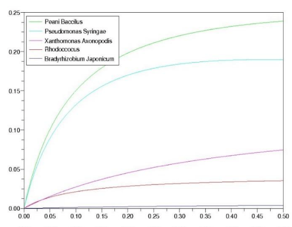
2.3.2 Growth rate estimation: We suppose that, initially, there was no dead cell, and that at exponential phase, the natural mortality is negligible. We calculated, for each glucose concentration, the regression coefficient at exponential phase, we obtained growth rate of all strains as functions of glucose concentrations. The best-fit results based on the Monod equation were obtained using the “leastsq” routine available in Scilab software are presented hereafter (Figure 1).

The growth rate parameters are given hereafter (Table 1).

Results

3.1 Pure cultures

3.1.1 Parameter identification: The least squares method is used to identify model parameters by minimizing the following criterion :

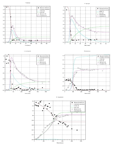
$J = \frac{σ_{1}}{2} \sum_{i = 1}^{n} s {(t_{i})}^{2} - s_{e} (t_{i}))^{2} + \frac{σ_{2}}{2} \sum_{i = 1}^{n} z_{e} (t_{i}) - z_{e} (t_{i}))^{2}$

where $t_{i}$ is the time variable, $s_{e}$ is the substrate concentration and $z_{e}$ is the optical density. $s (t_{i})$ and $z (t_{i})$ are the substrate and the optical density simulated using the model at time $t_{i}, i = 1, ..., n$ while $σ_{1}$ and $σ_{2}$ are weighting coefficients. A good fitting is observed in spite of noises present in available data (Figure 2, Table 2).

3.2 Mixed cultures

3.2.1 Extended model: In the present paragraph, the model is modified for the case of many cells in the same culture. For $i = 1, ..., n, x_{i}$ denotes the th viable cell concentration, $x_{d i}$ the ith non-viable cell concentration and s the substrate concentration. The mathematical model for n species is described by the following equation based on model (1) :

${\begin{array}{l} \dot{s} & = - \sum_{i = 1}^{n} \frac{μ_{i} (s)}{Y_{i}} x_{i} + \sum_{i = 1}^{n} λ_{i} (1 - δ_{i}) m_{i} x_{i} \\ {\dot{x}}_{i} & = (μ_{i} (s) - m_{i}) x_{i} \\ _{\dot{x} d i} & = δ_{i} m_{i} x_{i} \end{array}$

Such that

$\frac{1}{Y_{i}} > λ_{i}, i = 1... n .$

Assume that for t=0, there is no non-viable cells, then the following initial conditions :

$s (0) = s_{0} > 0, x_{d i} (0) = 0, x_{i} (0) = x_{i 0} > 0$

and

$μ_{i} (s) = μ_{m a x i} \frac{s}{k_{s}^{i} + s}, i = 1, n$

where $μ_{m a x i}$ and $k_{s i}$ are respectively the maximum growth rate and the saturation constant for the th species. The parameters $Y_{i}, λ_{i}, δ_{i}, m_{i}, μ_{m a x i}$ and $k_{s i}$ are identified at batch culture and are given in Paragraphs 2.3.2 and 3.1.1.

3.2.2 Optical density and substrate measurments: Available measurements are the substrate concentration and the optical density modelled as a linear combination of viable and non-viable cells concentrations of all strains in the culture and it is defined hereafter

$z = \sum_{i = 1}^{n} (γ_{1 i} x_{i} + γ_{2 i} x_{d i})$

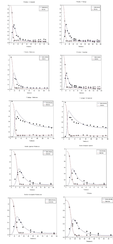
where the models parameters andare the absorptivity coefficients and are identified at batch culture and are given in paragraph 3.1.1 (Figure 3).

Discussion and Conclusion

Models of batch culture focus most of the time on the exponential growth phase (and its previous lag phase), when the substrate is non limiting. Cell mortality is usually neglected during these phases. Here we show that mortality cannot be neglected when one wants to study the growth after the exponential growth, i.e. when the substrate becomes limiting (as it is most probably the case in true soil ecosystems). Then, the model is close from continuous culture or chemostat ones, mortality playing the role of the dilution rate.

For chemostat models, many works have been achieved about the Competitive Exclusion Principle (CEP), stating that at most one species can survive on the long term [5-15]. Some of them tend to show that it is not valid in natural ecosystems (see for instance the [16]. On the opposite, other ones tend to show that it is valid in perfectly controlled environment [17]. One of the crucial questions in ecology is to decide if the invalidity of the CEP is due to intrinsic interactions between species or interactions with their environment. In the first case, the usual chemostat model on which the CEP is based is invalidated, and one has to take into account additional interaction terms. In the second case, one may conclude that the domain of validity of the model is not met but cannot a priory reject the model. Our experiments have been conducted in a framework similar to the the one driven in [17] and consequently tend to show that the CEP is also valid for the particular artificial consortia we have considered. Although some studies point out the role that could play complex interactions in the functioning and performances of simple artificial ecosystems (under quite the same conditions than ours), it is expected that bacteria of an artificial consortia - do not develop such a network of complex interactions. Let us also point out that all the species we have considered present quite different break-even concentrations. It is well known that the prediction of CEP requires more time to be observed when species have close break-even concentrations [12], as this may be the case when considering ecosystems with a huge number of different species in non negligible quantities [18-20]. We have avoided here such situations.

The Bioscreen machine automated bacterial growth curves by measuring the optical density. Their values are linear to the bacterial concentration values at exponential phase but it can’t describe the behaviour on the other phases. We proposed a mathematical model, validated on experimental data aiming at describing and predicting microbial growth on an essential limited substrate in batch pure cultures in revisiting the way where the optical density is modelled. This model takes into account viable cell growth, substrate consumption, cell mortality, non-viable cell accumulation in the culture medium and partial dead cell recycling into substrate. This model uses the optical density poor information at exponential phase to predict the behaviour for all phases. The least squares method is used to identify the model parameters. The system is then extended and validated on mixed cultures proving that there is only competition for the substrate which goes a little against the current thought relative to the complexity of the biological systems. Perspectives include co-cultures modelling in non-homogeneous media.

Aknowledgement

The experimental data has been achieved within the BIOCOM-MSE-UMR, INRA, Dijon, France. I am grateful to MSE for its technical and human support.

References

Copyright

© 2019 Hajji ME. This is an open-access article distributed under the terms of the Creative Commons Attribution License, which permits unrestricted use, distribution, and reproduction in any medium, provided the original author and source are credited.

View Similar Articles

Share your thoughts and experiences

Article Alerts

Subscribe to our articles alerts and stay tuned.

This work is licensed under a Creative Commons Attribution 4.0 International License.

Quick Enquiry

Nomenclature
t_i [h]	Time
χ, χⁱ [g/L]	Viable cell concentration
χ^d, χ^di [g/L]	Non-viable cell concentration
s [g/L]	Substrate concentration
se [g/L]	Measured substrate
Z	Calculated optical density
ze	Measured optical density
χ^s, χ^si [g/L]	Saturation constant
y, yi	Biomass yield coefficient
m, mi [h-1]	Mortality rate
m, mi [h-1]	Specific growth rate
μmax μmaxi	Maximum growth rate
δ, δi	Dead cell accumulation coefficient
λ, λi	Biomass conversion to substrate yield coefficient
γ¹, γ¹ⁱ , γ², γ²ⁱ	Specific absorptivity coefficient

Bergersen medium
Di-sodium Hydrogen Phosphate	0.45 g/L
Magnesium Sulphate	0.1 g/L
Ferric Chloride	0.02 g/L
Calcium Chloride Dihydrate	0.05 g/L
Yeast Extract	0. 5 g/L
Biothine	2mg/L
Thiamine	1mg/L
Glucose

Inocula	Phylogenetic affiliation
Peani baccilus	Firmicutes Bas GC
Pseudomonas syringae: PV. Tomato PT23	γ-proteobacteria
Xanthomonas axonopodis : C7R12	γ-proteobacteria
Rhodococcus : ATCC 13898 R27	Actynomycetales Haut GC
Bradyrhizobium japonicum	a-proteobacteria

Table 1: Growth rate parameters.
Strain - Parameters	mµmax	k_s
Peani Baccilus	0.208153	0.1
Pseudomonas syringae	0.124564	0.1
Xanthomonas axonopodis	0.108606	0.16
Rhodococcus	0.043493	0.21773
Bradyrhizobium japonicum	0.0075893	.503239

Table 2: Model parameters
Strain	γ	δ	λ	m	γ¹	γ²
Peani Baccilus	1.026	0.107	0.197	0.1	0.67	0.371
Pseudomonas syringae	1.164	0.137	0.718	0.1	0.68	0.49
Xanthomonas axonopodis	1.139	0.01	0.85	0.1	0.64	0.443
Rhodococcus	1.003	0.99	0.197	0.136	0.103	2
Bradyrhizobium japonicum	1.34	0.975	0.464	0.1	0.702	0.895

Open Journal of Environmental Biology

How the competitive exclusion principle can be validated using optical density measurements collected on artificially reconstituted soil ecosystems

Miled EL Hajji*

Author and article information

Abstract

Main article text

Introduction

Material and Method

2.1 Experimental process

2.2 Mathematical model: an extension of the Monod’s one

2.3 Available data

Results

3.1 Pure cultures

3.2 Mixed cultures

Discussion and Conclusion

Aknowledgement

References

Copyright

View Similar Articles

Share your thoughts and experiences

Article Alerts

Table of Contents

Submit your next article Peertechz Publications, also join of our fulfilled creators. Submit a Manuscript

© Peertechz Publications Inc., 10880 Wilshire Blvd., Suite 1101, Los Angeles, California, 90024, USA