Corrosion Detection in Pipelines Based on Measurement of Natural Frequencies

Zhenghao Yang; Erkan Oterkus; Zhenghao Yang; Erkan Oterkus

ISSN: 2641-3078

Annals of Limnology and Oceanography

Research Article Open aaacess Peer-Reviewed

Corrosion Detection in Pipelines Based on Measurement of Natural Frequencies

Zhenghao Yang and Erkan Oterkus*

Author and article information

University of Strathclyde, UK

*Corresponding author: Dr. Erkan Oterkus, 100 Montrose Street Glasgow, University of Strathclyde, G4 0LZ United Kingdom, Tel: +44-771-470-3872; E-mail: erkan.oterkus@strath.ac.uk

DOI: 10.17352/alo.000004

Received: 31 December, 2016 | Accepted: 21 January, 2017 | Published: 24 January, 2017

Keywords: Corrosion detection; Pipeline; Rayleigh’s law; Natural frequency

Cite this as

Yang Z, Oterkus E (2017) Corrosion Detection in Pipelines Based on Measurement of Natural Frequencies. Ann Limnol Oceanogr 2(1): 001-006. DOI: 10.17352/alo.000004

Abstract

Natural frequency of structure mainly depends on mass and stiffness. Stiffness is bound to change after structural damage. Hence, natural frequency starts to decline.

This study presents a new method to determine the location and degree of the corrosion damage by measuring the natural frequencies of the damaged pipeline. With this method, only measurement of the first and second natural frequencies of damaged pipeline is required. The formulation is based on Rayleigh’s Law to determine a relationship between the degree of damage and damage location. The formulation is validated by comparing against beam and solid finite element models.

Main article text

Introduction

Pipeline transport is important in modern industry, and pipelines are widely used in the fields of petroleum, natural gas, coal gas, chemical fluid, water, coal, etc. They are especially common in the petrochemical and natural gas industries. Furthermore, urban water supplies and gas systems, which are an integral element of modern society, rely on even larger pipeline networks. Various factors, including pipeline corrosion, external force and loose joint parts, may lead to pipeline leaks. Such leaks result, not only in resource consumption and economic loss, but also serious environmental pollution. In order to avoid pipeline accidents, there is a distinct requirement for systems by which industrial pipelines can be monitored on a real-time basis and safety assessments and durability predictions can be produced. The two main challenges associated with the online monitoring of pipeline operations are the detection of pipeline defects and the accurate identification of the location of the pipeline damage.

Structural damage results from a variety of different factors including operation overload, impingement, cracks, corrosion, strains, production defects, etc. These deficiencies will often lead to changes in the physical properties (rigidity, mass, damping) of a structure and will be accompanied by changes in its dynamic behaviours. This fact is commonly acknowledged in processes that involve monitoring the health of engineering structures and identifying any damage. Pipeline systems, which are part of large-scale structural engineering applications, are a fundamental element of lifeline engineering; therefore, significant attention has been invested in processes by which any damage to a given pipeline structure can be rapidly and accurately detected. When the operation of a pipeline structure exceeds a certain amount of time, its structure can be measured dynamically with the help of vibration testing. The dynamic behaviours of the data obtained can subsequently be employed to assess the overall health of the pipeline structure. Also, this form of detection, which is based on vibration features, has already been applied to assess various other structures including bridges, architecture, etc. Along with the development of modern sensor technology, microelectronics and computer technology, data collection, transmission, real-time analysis and processing technology have also been used widely. Vibration testing technology represents an automated and miniaturized detection system and, as a result, the detection of structural damage through the assessment of dynamic behaviours has consistently been a hot topic in the international academic community as well as within engineering circles. Coupled with the development of Finite Element Theory, it is anticipated that damage detection based on vibration technology will play a much more prominent role in the future [1-3].

At present, vibration methods are widely used to detect the corrosion of engineering structures. Some of the existing techniques are based on studying changes in vibration mode shape or damping factors. For example, Vitaly and Vladislav [4], developed a method of monitoring the vibration distortions that could be observed in a system’s symmetry as a result of the development of defects. Panteliou [5] and Kyriazoglou [6], investigated the effects of vibration damping factors on crack detection. Another approach to corrosion detection is based on monitoring changes in resonant frequencies. For example, Liang [7] and Barad [9], employed a natural frequency method by starting with a differential equation of free vibration [4-10].

This study describes a new corrosion detection method that involves the measurement of natural frequencies using an approach that is based on Rayleigh’s Law. This method is sampled on a pipeline and employed to assess the relationship between the location of the corrosion and degree of corrosion by adopting sectional integration and integral transformation. The main advantage of this approach is its simplicity while allowing a more accurate detection of the location of damage than the traditional natural frequency method.

Procedures for the development of the corrosion detection method

The use of Rayleigh’s Law to calculate natural frequency is based on the principle of the conservation of energy. When an elastic body is free of vibration without damping, its total mechanical energy (sum of strain energy and kinetic energy) remains constant.

For a distributed mass beam with a uniform section, its displacement function can be given by:

$y (x, t) = Y (x) sin (ω t + α) (1)$

where $Y (x)$ is the amplitude, ω is the natural frequency, and ω and $α$ depend on initial condition. Natural frequency is the frequency at which the system oscillates without any external loading. Natural frequency of the structure mainly depends on mass and stiffness. To measure the natural frequency of a pipeline, a pulse analyzer system can be equipped with accelerometer sensors, which are used to conduct the structural dynamic vibration response for monitoring system and data acquisition [11].

The strain energy, U , of the free vibration beam can be expressed as:

$U = \frac{1}{2} \int_{0}^{L} E I {[y (x)'']}^{2} d x = \frac{1}{2} s i n^{2} (ω t + α) \int_{0}^{L} E I {[Y'' (x)]}^{2} d x (2)$

where 1 is the length of the beam, E is the elastic modulus, andis the moment of inertia.

Moreover, kinetic energy, T can be expressed as:

$T = \frac{1}{2} \int_{0}^{L} ρ A {[\dot{y (x, t)}]}^{2} d x = \frac{1}{2} ω^{2} c o s^{2} (ω t + α) \int_{0}^{L} ρ A {[Y (x)]}^{2} d x (3)$

The strain energy reaches a peak value when the beam has the maximum amplitude; meanwhile, the kinetic energy is 0. When the amplitude is 0, the kinetic energy has the maximum value; meanwhile, the strain energy is 0. The maximum strain energy, $U_{\max}$ , and kinetic energy, $T_{\max}$ , can be respectively given as:

$U_{m a x} = \frac{1}{2} \int_{0}^{L} E I {[Y^{''} (x)]}^{2} d x (4a)$

and

$T_{m a x} = \frac{1}{2} ω^{2} \int_{0}^{L} \bar{m} {[Y (x)]}^{2} d x (4b)$

where $\bar{m}$ is the mass per unit length.

According to the principle of conservation of energy, we have $U_{\max} = T_{\max}$ , hence:

$ω^{2} = \frac{\int_{0}^{Λ} Ε Ι {[Ψ^{∍ ∍} (ξ)]}^{2} δ ξ}{\int_{0}^{Λ} \bar{μ} {[Ψ (ξ)]}^{2} δ ξ} (5)$

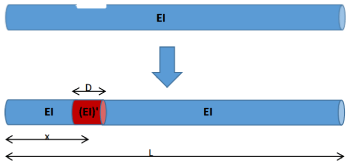
When considering a corroded pipeline, it can be assumed that the corrosion pit decreases the bending stiffness at the damaged position of the pipe, as shown in Figure 1,

where EI and (EI)’ are the bending stiffnesses of the intact and corroded elements of the pipe, respectively, L is the length of the pipe, x is the distance between the midpoint of the corroded segment to the left end of the pipeline, and D is the length of the corroded segment. If we neglect the mass loss due to the corrosion and apply these parameters into Eq. (5), the natural frequency of the corroded pipe can be obtained as follows:

$ω_{c}^{2} = \frac{\int_{0}^{x - D / 2} E I {[Y'' (x)]}^{2} d x + \int_{x - D / 2}^{x + D / 2} {(E I)}^{'} {[Y'' (x)]}^{2} d x + \int_{x + D / 2}^{L} E I {[Y'' (x)]}^{2} d x}{\int_{0}^{L} \bar{m} {[Y (x)]}^{2} d x} (6)$

If we introduce a factor, c, to describe the degree of the corrosion pit, where, $c = (E I)' / (E I)$ Eq. (6) can be rewritten as:

$ω_{c}^{2} = \frac{\int_{0}^{L} E I {[Y (x)'']}^{2} d x - \int_{x - D / 2}^{x + D / 2} (1 - c) E I {[Y (x)'']}^{2} d x}{\int_{0}^{L} \bar{m} {[Y (x)]}^{2} d x} (7)$

$ω_{c}^{2} = ω_{I}^{2} - \frac{(1 - c) E I}{\bar{m}} \cdot \frac{\int_{x - D / 2}^{x + D / 2} {[Y (x)'']}^{2} d x}{\int_{0}^{L} {[Y (x)]}^{2} d x} (8)$

where $ω_{I}$ is the natural frequency of the intact pipe with the same dimensions. Then, the degree of corrosion, c, can be represented by the following expression:

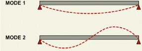
$c = \frac{(E I)'}{E I} = 1 - \frac{\bar{m} (ω_{I n}^{2} - ω_{C n}^{2})}{E I} \cdot \frac{\int_{0}^{L} {[Y_{n} (x)]}^{2} d x}{\int_{x - D / 2}^{x + D / 2} {[Y_{n} (x)'']}^{2}} (9)$

Here ‘n’ is the nth vibration mode, ωIn and ωCn are the nth natural frequenies of the intact and corroded pipe, respectively, and $Y_{n} (x)$ is the nth vibration mode function. The research presented in this study is based on examples of a simply supported constrain and the first and second mode of vibration for this boundary condition is shown in Figure 2 [12].

Thus, the vibration mode functions of the first two modes can be expressed as:

$Mode 1 : Y_{1} (x) = a_{1} \sin (\frac{π x}{L}) (10a)$

$Mode 2 : Y_{2} (x) = a_{2} sin (\frac{2 π x}{L}) (10b)$

If corrosive length, D, can be estimated to a reasonable level, by combining Eqs. (9), (10a) and (10b), the extent of corrosion factor, c, and corrosion location, x, can be predicted in consideration of the natural frequency of the intact pipeline ωI, and the corroded pipeline ωc.

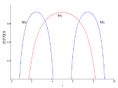
For example, a corroded pipeline with simply supported constrains has the following properties: pipe length L = 10 m, Young’s modulus E = 210 GPa, mass density ρ = 7850 kg/m3, 0.25 m of outer radius, and 0.02m of thickness. Its first and second natural frequencies were measured as ωc1 =53.89rad/s and ωc2 =213.69rad/s, and its corresponding natural frequencies of intact pipeline were calculated using Eq. (5) as: ωI1 =55.81Rad/s and ωI2 =221.30Rad/s, and corrosion length was assumed to be D = 0.50 m, then the variation of c with corroded region position x was plotted and is presented in Figure 3. Since physically there is only one unique c value to represent the degree of corrosion at the damaged locations, the potential corrosion region positions are denoted by the intersection points of the curves (Figure 3), and the numerical value of c at the intersection points represents the degree of pipeline corrosion. Due to the symmetry of this pipeline structure, there are two intersection points at about x =3. 30 m and x = 6.70 m and the actual corrosion region position is one of them.

Finite element analyses

In order to investigate and verify the accuracy of the pipeline damage detection through the use of natural frequency measurements, a commercial finite element program, ANSYS, was employed.

A simply supported corroded pipeline was modelled using Beam188 element with the following characteristics: Pipeline length, L=10 m outer radius, r = 0.16 m wall thickness, t = 0.01m mass density $ρ = 7850$ kg/m3, elastic modulus of non-corroded segment, E = 210 GPa elastic modulus of corroded segment E’ = c . E. Here, c represents the degree of corrosion, ranging from 0 to 1. The model was discretized with 20 elements along the axis, as shown in Figure 4. Five simulation cases were analysed with five different corrosion positions and corrosion levels. Their first and second natural frequencies, ωC1 and ωC2 , were computed individually using ANSYS, as shown in Table 1.

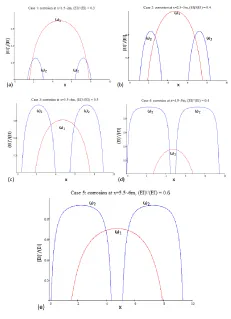
Based on the first and second natural frequencies that were computed using ANSYS ( 1) and the corresponding natural frequencies of the intact pipeline, $ω_{I 1} = 55.81 rad / s, ω_{I 2} = 221.30 rad / s$ , Eq. (9) can be solved to determine the variation of (EI’/EI) versus the location of the corrosion for the first two modes. The results of Cases 1 to 5 are shown in Figure 5, which depict the location of the corrosion and the degree of corrosion at the intersection points. There are two intersection points in each graph and this is due to the symmetry of the structure. The solution and plots were calculated using Mathcad.

As can be seen clearly from Table 2, the calculations in terms of the location of the corrosion and the degree of corrosion were accurately predicted.

It is noteworthy that, from the characteristic Eq. (9), there is an important parameter, the effect of estimated corrosion length ‘D’, which should not be neglected. The FEA described above reveals that, ideally, if an estimated ‘D’ is merely equal to the practical corrosion length, both corrosion location and degree of corrosion can be accurately predicted. However, in practical engineering applications, it is almost impossible to accurately estimate corrosion length. Thus, it is also important to take into consideration the estimated corrosion length, ‘D’, in order to investigate how this affects the prediction.

A further finite element analysis was carried to investigate the influence of ‘D’. The finite element model was largely based on Case 3 of the previous problem. The only changes were that the corrosion segment was increased to 1 m, and the midpoint of the corrosion was positioned at x = 3.50 m, as shown in Figure 6.

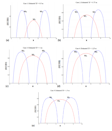
The first two natural frequencies of this corroded pipeline were computed using ANSYS, and were $ω_{C 1} = 51.86 rad / s$ and $ω_{C 2} = 209.93 rad / s$ . A total of five cases of varying values of ‘D’ were incorporated into the characteristic, Eq. (9). These were D = 0.50 m, 0.75 m, 1 m, 1.25 m and 1.5 m. The results of Cases 1 to 5 were calculated using Mathcad, as shown in Figure 7, and detailed data is presented in Table 3.

As can be clearly seen from Table 3, in all cases, the corrosion position were predicted correctly, even though the predicted corrosion length, D, was smaller or greater than the actual corrosion length. However, over or under estimating D will affect the accuracy of the predicted degree of corrosion.

Finite element analyses of other geometries

In order to expand the investigation of the current corrosion detection method, a 3D corrosive pipeline model was studied using ANSYS, and this model was deemed to be more reflective of reality.

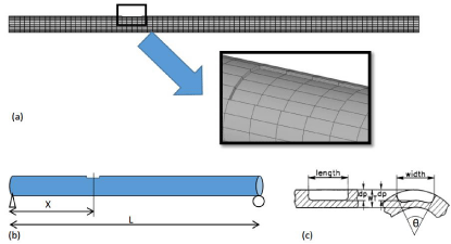
The finite element model was designed with a 20-node isoparametric Solid186 element. The length was 10 m, the inner and outer radius of the pipe were RI = 0.18 m and RO = 0.2 m, the elastic modulus was E=210 GPa, mass density ρ = 7850 kg/m3, and the Poisson ratio ν = 0.3. There were 24 cells along the circumference, 5 cells along the thickness, and 80 along the axis. The corrosion pit was idealized into a rectangular shape, and a typical finite element mesh is shown in Figure 8a.

Four different parameters of,x l_c , dp and () were considered in the FEA. Here, x represents the location of the corrosion in terms of the distance from the left end of the pipeline to the midpoint of the dp corrosion pit; represents the length of the corrosion pit; l_c dp represents the depth of the corrosion pit, anddescribes the width of the corrosion pit. As shown in Figure 8b,c, all four cases were studied by varying the above parameters as summarized in Table 4.

The constraints of the two ends of the finite element model were set to be simply supported. For all cases, the first and second natural frequency, ωC1and ωC2, were computed with the help of ANSYS, and the corresponding dimensional intact pipeline model was also created by using ANSYS to compute its first and second natural frequency, ωI1and ωI2. The details of FEA results are summarized in Table 5.

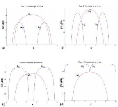
The computed natural frequencies are given in Table 5 by using an estimated corrosion length of D = 0.5 m. This information was plugged into Eq. (9) to calculate the variation of corrosion degree (EI)’/(EI) versus the corrosion pit location. Evaluated results are presented in Figure 9. The intersection points represent the corrosion pit location and the corrosion degree. Again, due to the symmetry, there are two potential corrosion locations for Case 1-4, and the actual location is at one of them.

The numerical results for all cases are shown in Table 6. This data clearly indicates that the predictions of the corrosion pit location are pretty accurate and that there is a good agreement between the finite element model and the proposed method.

Moreover, this FEA more closely resembles reality because the corrosion is modelled by creating a pit on the wall of the pipeline rather than decreasing the flexural rigidity of a segment. However, it can be simply estimated based on common sense that the larger and deeper the corrosion pit is, the more serious the degree of corrosion. According to the corrosion pit dimensions of each case, the degree of corrosion sequence from high to low is Case 2 < Case1 < Case 3 < Case 4, and this rank is reflected by the given results.

Discussion and Conclusions

This study presents a new method for detecting corrosion damage within a pipeline structure that is based on measurements of first and second natural frequency. The method is based on Rayleigh’s Law to determine a relationship between c (degree of corrosion) and corrosion location. Since only one unique value of c is physically permissible at a given corrosion location, the intersections of the various values of c at various natural frequencies along the axial direction of the pipeline provided insights into the location of the corrosion damage.

Two different types of finite element models were employed to verify the feasibility of this method: one considering the corrosion segment as a decreased bending stiffness on a uniform section pipeline, and the other using 3D Solid186 element within which the corrosion pit was modelled directly on the wall of the pipeline. More specifically, for the first type of model, the corrosion segment was created by decreasing its elastic modulus E, and the second model type by decreasing the moment of inertia. Both supported the application and accuracy of this method.

Note that an imprecise estimated value of corrosion length D does not affect the accuracy of the prediction of the corrosion location. However, it will lead to an inaccurate prediction of degree of corrosion. In this case, after determining the location of the corrosion, the length of the corrosion region should be measured in the pipeline and by using this actual length, Eq. (9) can provide an accurate degree of corrosion.

References

Copyright

© 2017 Yang Z, et al. This is an open-aaacess article distributed under the terms of the Creative Commons Attribution License, which permits unrestricted use, distribution, and reproduction in any medium, provided the original author and source are credited.

View Similar Articles

Share your thoughts and experiences

Article Alerts

Subscribe to our articles alerts and stay tuned.

This work is licensed under a Creative Commons Attribution 4.0 International License.

Quick Enquiry

Table 1: Parameters of FEM.
Case No.	Corrosion Position		Degree of corrosion
1	Element 4	x=1.50 ~ 2 m	0.30	54.07	203.86
2	Element 6	x=2.50 ~ 3 m	0.40	53.52	208.02
3	Element 8	x=3.50 ~ 4 m	0.50	53.58	216.34
4	Element 10	x=4.50 ~ 5 m	0.40	52.09	220.46
5	Element 12	x=5.50 ~ 6 m	0.60	54.14	219.74

Table 2: Comparison between prediction results and FEA results.
Case No.	Corrosion Location, x (m)	Predicted location, x (m)	Degree of corrosion, (EI)’/EI	Predicted degree of corrosion (EI)’/EI
1	1.50 ~ 2	1.70	0.30	0.23
2	2.50 ~ 3	2.80	0.40	0.38
3	3.50 ~ 4	3.70	0.50	0.48
4	4.50 ~ 5	4.50	0.40	0.37
5	5.50 ~ 6	5.70	0.60	0.64

Table 3: Comparison between prediction results and FEA results.
Case No.	Corrosion position and length, x(m), lc(m)	Degree of corrosion, (EI)’/(EI)	Estimated corrosion length, D(m)	Predicted corrosion position, x(m)	Predicted degree of corrosion, (EI)’/(EI)
1	x = 3.50 m lc = 1 m	0.50	0.50	3.57	0.15
2			0.75	3.53	0.45
3			1	3.55	0.52
4			1.25	3.57	0.63
5			1.50	3.54	0.70

Table 4: Parameters of finite element model.
Case No.	Pit location, x(m)	Pit length, lc(m)	Pit depth, dp(m)	θ(°)
1	2	0.75	0.012	90
2	3	0.75	0.012	120
3	4	0.50	0.010	90
4	5	0.50	0.010	60

Table 5: Natural frequency values from FEA.
Case No.	(rad/s)	(rad/s)	(rad/s)	(rad/s)
1	67.67	263.11	68.29	268.71
2	66.82	261.97
3	67.47	267.54
4	67.53	268.68

Annals of Limnology and Oceanography

Corrosion Detection in Pipelines Based on Measurement of Natural Frequencies

Zhenghao Yang and Erkan Oterkus*

Author and article information

Abstract

Main article text

Introduction

Procedures for the development of the corrosion detection method

Finite element analyses

Finite element analyses of other geometries

Discussion and Conclusions

References

Copyright

View Similar Articles

Share your thoughts and experiences

Article Alerts

Table of Contents

Submit your next article Peertechz Publications, also join of our fulfilled creators. Submit a Manuscript

© Peertechz Publications Inc., 10880 Wilshire Blvd., Suite 1101, Los Angeles, California, 90024, USA

Table 6: Comparison between prediction results and FEA results.
Case No.	Corrosion pit location, x (m)	Predicted location, x (m)	Degree of corrosion, (EI)’/(EI)	Degree of corrosion, (EI)’/(EI)
1	2	2.20	0.70	0.60
2	3	3.10	0.63	0.41
3	4	4	0.75	0.72
4	5	5	0.82	0.78